10  Relational Learning

Relational learning is the study of machine learning using expressive relational knowledge representation formalisms involving first-order logic. It targets relational problems, which are the ones involving multiple entities and relationships among them.

They use logic as a representation language for describing data and generalizations, because it is inherently relational, expressive, and interpretable. It allows us to specify and use background knowledge about the domain.

10.1 Representation

The learning goal is to discover hypotheses that provide information about the instances. Formally, it can be modeled by viewing hypotheses h \in L_h as functions h: L_e \rightarrow Y ranging on some domain Y. Language of examples and language of hypotheses can be different.

So, given:

• a language of examples L_e
• a language of hypotheses L_h
• an unknown target function f: L_e \rightarrow Y
• a set of examples E = (e_1, f(e_1)), \ldots, (e_n, f(e_n))), where e_i \in L_e
• a loss function loss(h, E)

We want to find the hypotheses h^* \in L_h such that

h^* = \argmin_{h \in L_h} loss(h, E)

The central definition is the coverage: c is a relation over L_h \times L_e, and c(h, e) = true if and only if h(e) = 1.

c is a matching relation, where c(h) is the set of examples in L_e covered by h \in L_h, and c(h, D) is the set of examples from D \subseteq L_e covered by h.

If we learn from entailment (implication), c(h, e) = true if e is entailed from h.

Different notions of coverage are possible, as well as choices for L_e and L_h.

10.2 Learning as Search

Symbolic Machine Learning techniques essentially search in a space of possible hypothesis L_h. The trivial algorithm is the Generate-and-Test algorithm, which essentially enumerates the hypotheses to find the best one.

for each h in L_h do
    if Q(h, D) = true then
        output h
    end if
end for

Whenever a solution exists, the algorithm will find it, but it can only be applied if the hypotheses language L_h is enumerable. We need to structure the search space in a smarter way.

We use the generality relation to prune the search space and guide the search towards promising parts of the space. A more general hypothesis logically entails the more specific one, a more specific hypothesis is a logical consequence of the more general one. So we can traverse the space using a general-to-specific direction, or the contrary.

Now we define generality between hypothesis. Let h_1, h_2 \in L_h. h_1 is more general than h_2, h_1 \preceq h_2 if and only if all examples covered by h_2 are also covered by h_1, that is, c(h_2) \subseteq c(h_1).

\preceq is transitive, reflexive but not anti-symmetric (quasi-order relation) since there may exist several hypotheses that cover exactly the same set of examples, that is, syntactic variants, which introduce redundancies in the search space.

We now define a quality criterion Q: L_h \times 2^{L_e} \rightarrow \{true, false\}, that is a function that evaluates the quality of a hypothesis with respect to a set of examples. We want to find the best hypothesis according to this criterion.

The generality relation imposes a useful structure on the search space provided that the quality criterion involves some properties, such as monotonicity: a quality criterion Q is monotonic if and only if \forall s, g \in L_h, \forall D \subseteq L_e: (g \preceq s) \land Q(g, D) \rightarrow Q(s, D), this allows a top-down search, while if it is anti-monotonic (Q(s, D) \rightarrow Q(g, D), maintaining the other conditions) it allows a bottom-up search.

Directly following from the definitions of monotonicity and anti-monotonicity:

• If a hypothesis h does not satisfy a monotonic quality criterion then none of its generalizations will.
• If a hypothesis h does not satisfy an anti-monotonic quality criterion then none of its specializations will.

These properties allow us to prune the search space.

To traverse the space many algorithms rely on refinement operators, that are, operators that generate a set of specializations (or generalizations) of given hypotheses:

• Generalization operator p_g: L_h \rightarrow 2^{L_h} is a function such that \forall h \in L_h: p_g(h) \subseteq \{ h^{'} \in L_h | h^{'} \preceq h \}

• Specialization operator p_g: L_h \rightarrow 2^{L_h} is a function such that \forall h \in L_h: p_g(h) \subseteq \{ h^{'} \in L_h | h \preceq h^{'} \}

p is an ideal operator iff it returns all proper refinements and not a syntactic variant of the original hypothesis.

p is an optimal operator if \forall h \in L_h there exists exactly one sequence of hypotheses T = h_0, \ldots h_n = h \in L_h such that h_i \in p(h_{i - 1}) for all i. No hypothesis will be generated more than once when starting from h_0.

An operator for which there exists at least one sequence from T to any h \in L_h is called complete.

An operator for which there exists at most one sequence from T to any h \in L_h is non-redundant.

10.2.1 Generic Algorithm

Adapting the enumeration algorithm to employ the refinement operators, we are effectively representing a lot of algorithm with a single formulation:

q = INIT(queue)
thesis = []
while not STOP
    h = q.DELETE()
    if Q(h, D) then
        thesis.append(h)
        q.add(p(h))
    end if
    q = prune(q)
end while
return thesis

• INIT determines the starting point for a bottom-up or a top-down approach
• DELETE determines the search strategy
  • FIFO: BFS (to avoid infinite paths)
  • LIFO: DFS (if branching factor is high)
  • Best-first algorithm (heuristic)
• p determines the size and nature of the refinement steps
• STOP determines the stop condition
• PRUNE determines which algorithms are used to prune candidate hypotheses
  • heuristic pruning prunes away unpromising paths
  • sound pruning prunes away parts of the search space that cannot contain solutions
• Complete algorithms compute all elements of the thesis
• Heuristic algorithms aim at computing one of a few hypotheses that score best with respect to a given heuristic, without guarantee to find the best hypotheses.

10.3 Description Logics

Description logics is a family of logics of different expressive power all derived from decidable fragment of first-order logic. It describe the domains in terms of concepts (classes), roles (relation) and individuals.

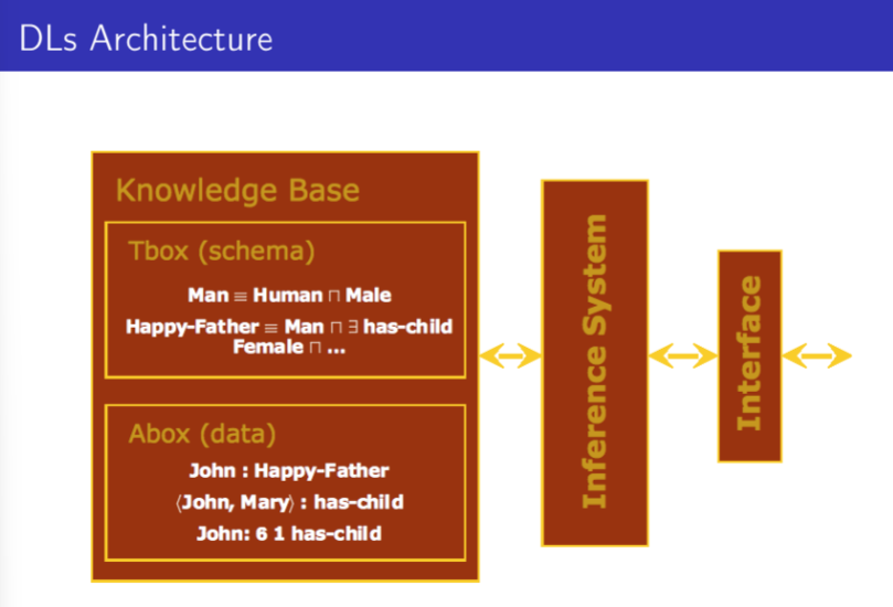
A Knowledge base is a pair \mathbf{K} = (\mathbf{T}, \mathbf{A}):

• T is called T-box and is the set of terminological axioms
  • Operators are subsumption (D \sqsubseteq C) and definitions A \equiv D
• A is called A-box and is a set of assertional axioms C(a), R(a, b)
  • An interpretation \mathbf{I} satisfies C(a) and R(a, b) if a^I \in C^I and (a^I, b^I) \in R^I

An interpretation \mathbf{I} is a model of \mathbf{K} if every axiom is satisfied by \mathbf{I}

Let be C and D two concept descriptions, C subsumes D (D \sqsubseteq C) iff for all interpretations \mathbf{I}, D^I \subseteq C^I.

Two concepts are equivalent (C \equiv D) if for all interpretations \mathbf{I} we get C^I = D^I.

Given a DL KB the implicit knowledge may be made explicit by reasoning operators such as:

• Concept subsumption: assess if a concept is more general/specific than another one
• Instance checking: decide whether an individual is an instance of a concept
• Retrieval: find all individuals that are instances of a concept

In KB we use the Open World Assumption: missing information is interpreted as information not known, while in DB and ML we use the Closed World Assumption.

10.3.1 Concept Learning in Description Logics

Given:

• a Knowledge Base
• a target concept C
• a set of positive and negative examples E = E_{+} \cup E_{-} for C

We want to find a description D for C generalizing E, C \equiv D, that maximizes the accuracy with respect to the positive and negative examples.

Accuracy: a description D correctly entails at least (1 - \epsilon) |E| of the assertions on examples regarding their membership to C:

\forall e \in E_+: \mathbf{K} \sqcup \{d\} \vDash C(e) \land \forall e \in E_-: \mathbf{K} \sqcup \{d\} \not\vDash C(e)

A stronger alternative aims to demonstrate that every negative example is not logically entailed (\mathbf{K} \sqcup \{D\} \vDash \neg C(e)).

The idea is to randomly and recursively generate new refinement operator adding a conjunction to the operators already available.

An algorithm used for this is DLFoil, a heuristic sequential covering algorithm, that employs a general-to-specific search:

• Starting from \top
• repeat (cover as many positives as possible)
  • if non positives are covered
  • repeat
    • find heuristically the best refinement (not to cover them yet still covering as many positives as possible)
    • add refinement as a disjunct partial def.
  • until only positives covered
• until all positives covered

The heuristic function is:

g(D_0, D_1) = p_1 \cdot \left[ \log \dfrac{p_1}{p_1 + n_1 + u_1} - \log \dfrac{p_0}{p_0 + n_0 + u_0} \right]

• p are the positive examples
• n are the negative examples
• u are the unknown examples
• p_1, n_1, u_1 are the number of examples covered by the definition D_1
• p_0, n_0, u_0 are the number of examples covered by the former partial definition D_0
• we add the Laplace smoothing